Optimization Metrics Reference

What it is

The Optimization Summary Statistics table consolidates the most important metrics from your full parameter grid search into a single view. It answers three questions: how robust is the parameter space overall, what is the distribution of performance across all combinations, and does the best result show signs of overfitting?

This is often the best place to start when reviewing optimization results. Before diving into heatmaps, 3D surfaces, and individual analytics, the summary table tells you whether the optimization produced meaningful results worth investigating further — or whether the strategy concept needs rethinking.

How to access it

The Summary Statistics panel is displayed on the right side of the optimization analytics popup at all times — it remains visible regardless of which analytics tab is active on the left. Available on Plus plans and above (Deflated Sharpe requires Plus and above).

The optimization analytics popup is accessed via the table icon in the View Panel after your optimization job completes. See The Strategy Panel & View System for full details.

tip

Check % Profitable and % Sharpe > 1 first — a robust strategy works across a wide range of parameters, not just at a single peak. Then check Deflated Sharpe — if DSR is below 0.95, your best result may not survive out-of-sample testing despite looking good in the grid search.

What you see

The table is divided into five sections, each addressing a different dimension of the optimization results.

All distribution metrics (Best, Median, Worst, Std Dev across Sharpe, Return, and Profit Factor sections) operate on valid combinations only — combinations excluded by the minimum trade count threshold are removed before any metric is calculated.

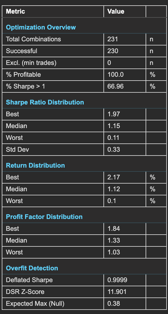
Optimization Overview

Basic counts and success rates across the full parameter grid.

Metric	Description
Total Combinations	Total parameter combinations tested in the grid search (e.g., 400 for a 20×20 grid).
Successful	Combinations that completed without errors. Failed combinations are excluded from all analytics.
Excl. (min trades)	Combinations excluded because they generated fewer than the minimum trade count threshold. These results are statistically unreliable and are removed from rankings and visualizations.
% Profitable	Percentage of all tested combinations that produced positive returns. A high % profitable (e.g., 100%) indicates a robust parameter space where the strategy works across a wide range of settings — not just at a single peak.
% Sharpe > 1	Percentage of combinations achieving a Sharpe ratio above 1.0. This is a more demanding robustness check than simple profitability — it requires risk-adjusted performance, not just positive returns.

Sharpe Ratio Distribution

How Sharpe ratios are distributed across the full parameter space.

Metric	Description
Best	Highest Sharpe ratio achieved across all combinations. This is the headline number — but it must be validated against the Deflated Sharpe before trusting it.
Median	Middle Sharpe ratio across all combinations. More representative of typical performance than the best. If the median is meaningfully positive, the strategy concept has broad validity.
Worst	Lowest Sharpe ratio across all combinations. Reveals the downside of poor parameter choices within your tested ranges.
Std Dev	Standard deviation of Sharpe ratios across combinations. Low std dev indicates a flat, robust parameter landscape where most combinations perform similarly. High std dev indicates a sharp peak — the "best" parameters are far better than the rest, which may indicate overfitting.

Return Distribution

Total return across the full parameter space.

Metric	Description
Best	Highest total return achieved across all combinations.
Median	Median total return across all combinations. This is the return you would expect from a randomly chosen parameter combination — your baseline expectation before parameter selection.
Worst	Lowest total return across all combinations. Can be significantly negative — shows the cost of choosing poor parameters.

Profit Factor Distribution

Profit factor (gross profit / gross loss) across the parameter space.

Metric	Description
Best	Highest profit factor across all combinations.
Median	Median profit factor across all combinations. Use this as your baseline expectation — a median above 1.0 means the typical combination is profitable on a win/loss basis.
Worst	Lowest profit factor across all combinations. Values below 1.0 indicate combinations where gross losses exceed gross profits.

Overfit Detection

Statistical tests that assess whether the best result is genuine or a product of testing many combinations.

Metric	Description
Deflated Sharpe	The Deflated Sharpe Ratio (DSR) corrects the best Sharpe ratio for multiple testing bias using the Bailey & López de Prado methodology. Values close to 1.0 (e.g., 0.9999) indicate the best result is statistically significant even after accounting for the number of combinations tested. Values below 0.95 warrant caution — the best result may not be genuine. Values are capped at 0.9999 — a DSR of 1.0000 would imply mathematical certainty of genuine edge, which is never appropriate.
DSR Z-Score	The z-score of the Deflated Sharpe test. Values above 1.28 indicate 90% confidence (DSR > 0.90). Above 1.65 reaches 95% confidence (DSR > 0.95). Above 2.33 reaches 99% confidence (DSR > 0.99). Since DSR = Φ(Z), confidence can also be read directly from the DSR value itself. Higher is better — a high z-score means the best Sharpe is far above what chance would produce.
Expected Max (Null)	The Sharpe ratio you would expect to find by chance given the number of combinations tested, assuming no real edge exists. Your best Sharpe should comfortably exceed this value. If your best Sharpe is close to Expected Max (Null), your result may be luck rather than edge — the optimizer found exactly what random variation would predict.

How the Deflated Sharpe Ratio works

When you test 400 parameter combinations and pick the best one, you are running 400 hypothesis tests and reporting the winner. The more combinations you test, the more likely it is that the best result is simply the luckiest. This is the multiple testing problem — the primary mechanism behind overfitting in strategy optimization.

The Deflated Sharpe Ratio (DSR), developed by Bailey and López de Prado, corrects for this bias by adjusting the observed Sharpe of the best combination.

The correction uses three inputs from the actual implementation:

• Number of valid combinations tested (K) — more combinations tested means a larger expected maximum Sharpe under the null hypothesis of no real edge
• Statistical properties of the best combination's returns — skewness and excess kurtosis of the best combination's trade P&L adjust the standard error of the Sharpe ratio following Lo (2002)
• Length of the best combination's trade record (T) — shorter records produce less reliable Sharpe estimates, making the correction more conservative when statistical backing is thin

Interpreting the Deflated Sharpe

Deflated Sharpe	Assessment
Above 0.95	Strong evidence of genuine edge. The best result holds up statistically even after accounting for the number of combinations tested.
0.5 – 0.95	Moderate evidence. Consider additional validation via walk-forward optimization before trusting the result.
Below 0.5	Weak evidence. The best Sharpe is largely explainable by testing many combinations. Treat with caution.
Near zero or negative	No meaningful signal found. The optimizer found what random variation would predict.

Key comparison — raw vs deflated: A modest deflation (e.g., raw 1.82 → deflated 1.45) means the result is robust. A severe deflation (e.g., raw 1.82 → deflated 0.35) means most of the observed performance is attributable to testing many combinations, not genuine edge.

The DSR Z-Score and Expected Max (Null) provide additional context: your best Sharpe should comfortably exceed the Expected Max (Null), and a Z-Score above 1.65 reaches 95% confidence that the result is not luck.

Metric Formulas

Every formula below is extracted directly from compute_optimization_metrics(). All calculations operate on valid combinations only — combinations excluded by the minimum trade count threshold are removed before any metric is calculated.

For formulas covering Sharpe Ratio, Profit Factor, Total Return, Win Rate, Max Drawdown, Calmar Ratio, Volatility, and Win/Loss Ratio see Backtest Metrics Reference.

---

% Profitable

              # combinations where total_return > 0
% Profitable = ─────────────────────────────────────── × 100
                            N_valid

Variables:

• N_valid = combinations meeting the minimum trade threshold
• total_return = Total Return (%) per combination

Platform convention: Strictly greater than zero — breakeven combinations count as unprofitable. Denominator is valid combinations only, not total combinations tested.

---

% Sharpe > 1

              # combinations where sharpe_ratio > 1.0
% Sharpe > 1 = ──────────────────────────────────────── × 100
                             N_valid

Variables:

• N_valid = valid combinations (same filter as % Profitable)
• sharpe_ratio = annualised Sharpe ratio per combination

Platform convention: Threshold is strictly greater than 1.0. Same denominator filter as % Profitable.

---

Sharpe Distribution (Best / Median / Worst / Std Dev)

  col    = { sharpe_i : combination i is valid, i = 1 … N_valid }

  Best   = max(col)
  Median = median(col)
  Worst  = min(col)

             1
  Std Dev = ─────  Σ (sharpe_i − sharpe_mean)²    ← sample std (ddof=1)
            N − 1

Variables:

• sharpe_i = Sharpe ratio of combination i
• sharpe_mean = mean Sharpe across valid combinations
• N_valid = number of valid combinations

Platform convention: Sample standard deviation (divides by N−1). The same Best/Median/Worst structure applies identically to the Return and Profit Factor distributions using total_return and profit_factor respectively.

---

Expected Max Sharpe (Null) — SR*

Step 1 — Standard error of the best Sharpe (Lo 2002):

            ┌─────────────────────────────────────────────────────────┐
            │  1 − γ₁ × SR_best + ((κ + 2) / 4) × SR_best²          │
  SE(SR) = √│ ────────────────────────────────────────────────────── │
            │                       T                                 │
            └─────────────────────────────────────────────────────────┘

Step 2 — Expected maximum z-score under the null:

  E[Z_max] = (1 − γ_e) × Φ⁻¹(1 − 1/K)  +  γ_e × Φ⁻¹(1 − 1/(K×e))

Step 3 — Expected max Sharpe in SR units:

  SR* = E[Z_max] × SE(SR)

Variables:

• SR_best = highest observed Sharpe across valid combinations
• γ₁ = skewness of the best combination's daily returns
• κ = excess kurtosis of the best combination's daily returns (normal = 0)
• T = number of trading days in the best combination's backtest period
• K = number of valid combinations (n_trials)
• γ_e = Euler-Mascheroni constant ≈ 0.5772156649
• e = Euler's number ≈ 2.71828
• Φ⁻¹(·) = standard normal quantile function (inverse CDF)

Platform convention: SR* is displayed as "Expected Max (Null)." Your best Sharpe should comfortably exceed SR*. If SR_best ≈ SR*, the optimizer found what statistical noise predicts.

---

DSR Z-Score

               SR_best − SR*
  Z_DSR  =  ─────────────────
                  SE(SR)

Variables:

• SR_best = highest observed Sharpe across valid combinations
• SR* = Expected Max Sharpe (Null) — see formula above
• SE(SR) = standard error of the best Sharpe — see formula above

Platform convention: Z_DSR is a standard normal z-score. Confidence thresholds:

  Z_DSR > 1.28  →  DSR > 0.90  →  90% confidence
  Z_DSR > 1.65  →  DSR > 0.95  →  95% confidence
  Z_DSR > 2.33  →  DSR > 0.99  →  99% confidence

Higher Z_DSR means the best observed Sharpe is further above what chance predicts.

---

Deflated Sharpe Ratio (DSR)

  DSR = Φ(Z_DSR)

Variables:

• Φ(·) = standard normal cumulative distribution function
• Z_DSR = DSR Z-Score as defined above

Platform convention: Result is bounded to [0, 0.9999] — a cap of 0.9999 prevents display of DSR = 1.0000, which would falsely imply mathematical certainty of genuine edge.

DSR is a probability: a DSR of 0.9987 means there is a 99.87% probability that the observed best Sharpe exceeds what pure random testing of K combinations would produce under the null hypothesis of no real edge.

Academic reference: Bailey, D. H. & López de Prado, M. (2014). "The Deflated Sharpe Ratio: Correcting for Selection Bias, Backtest Overfitting, and Non-Normality." Journal of Portfolio Management, 40(5), 94–107.

The platform's implementation applies the Bailey & López de Prado framework. The exact implementation is not published.

How to interpret it

Quick assessment framework

Read the table top to bottom:

1. Optimization Overview answers: "Is the strategy broadly viable?" — % Profitable above 60% and % Sharpe > 1 in double digits is a strong start.
2. Sharpe Distribution answers: "What does the typical combination look like?" — Median Sharpe above 0.5 means the concept works broadly, not just at a peak.
3. Return and Profit Factor answer: "What should I expect?" — Median values are your baseline before parameter selection improves on them.
4. Overfit Detection answers: "Is the best result real?" — Deflated Sharpe above 0.95 and best Sharpe well above Expected Max (Null) together confirm the result.

Best vs. median gap

The gap between the best Sharpe and the median Sharpe indicates how much parameter selection matters:

• Small gap (best is less than 2× median) — Performance is stable across parameters. Any reasonable choice works. The parameter landscape is flat and robust.
• Large gap (best is more than 4× median) — Performance is highly parameter-dependent. The "best" result may be fragile. Check the Deflated Sharpe and Sharpe Std Dev to assess whether this is genuine edge or overfitting.

Profitability thresholds

% Profitable	Assessment
Above 80%	Excellent — the strategy concept is robust across nearly all parameter combinations
60–80%	Good — broad validity with some weak regions
40–60%	Mixed — parameter-sensitive, investigate which regions fail
Below 40%	Weak — most combinations lose, the strategy concept may not work on this instrument

Example

Summary statistics from a DEMA × EMA crossover optimization on BTC (400 combinations):

Optimization Overview:

• Total Combinations: 400
• Successful: 400
• Excl. (min trades): 0
• % Profitable: 61.5%
• % Sharpe > 1: 13.6%

Sharpe Ratio Distribution:

• Best: 1.82
• Median: 0.45
• Worst: −1.24
• Std Dev: 0.68

Return Distribution:

• Best: +7.99%
• Median: +1.82%
• Worst: −5.28%

Profit Factor Distribution:

• Best: 2.14
• Median: 1.18
• Worst: 0.42

Overfit Detection:

• Deflated Sharpe: 0.9987
• DSR Z-Score: 3.01
• Expected Max (Null): 1.41

Interpretation: 61.5% of combinations are profitable and the median Sharpe of 0.45 is meaningfully positive — the crossover concept has broad validity on BTC, not just isolated lucky combinations. The Deflated Sharpe of 0.9987 (essentially 1.0) with a z-score of 3.01 confirms the best result of 1.82 is statistically significant and well above the Expected Max (Null) of 1.41 — this is genuine edge, not luck from testing 400 combinations.

The gap between best (1.82) and median (0.45) Sharpe is notable — a 4× ratio — but the Deflated Sharpe confirmation and the 61.5% profitability rate together indicate the result is robust. The trader moves to Walk-Forward Optimization to confirm these results generalize to out-of-sample data.